多维熵动量趋势自适应交易系统


创建日期: 2025-08-18 17:12:33 最后修改: 2025-08-18 17:12:33
复制: 0 点击次数: 2
avatar of ianzeng123 ianzeng123
1
关注
134
关注者

多维熵动量趋势自适应交易系统 多维熵动量趋势自适应交易系统

概述

多维熵动量趋势自适应交易系统是一种基于熵理论的量化交易策略,核心是CETP-Plus指标,该指标通过Shannon熵测量蜡烛图模式中的”有序性”。该系统将指数移动平均线(EMA)的近期加权原理、相对强弱指标(RSI)的动量偏差、平均真实范围(ATR)的波动性缩放和平均方向指数(ADX)的趋势强度融合到单一评分中。这种独特方法避免了叠加多个指标的复杂性,同时提高了早期趋势检测的准确性和多空交易的平衡性。CETP-Plus通过将蜡烛图比率(实体、上下影线)分箱到三维直方图中计算熵值(低熵=强模式),并使用动量、波动性和趋势乘数调整得分以产生强健信号。当得分超过阈值时触发入场(正值做多,负值做空),在反转或止损时退出。该策略完全自动化,无需手动偏置,为保证金账户优化,对多空交易一视同仁。

策略原理

该策略的核心原理是将Shannon熵应用于金融市场蜡烛图模式分析。Shannon熵源自信息论,用于量化随机变量的不确定性或”混乱度”。在该策略中,通过以下方式计算和应用熵:

  1. 蜡烛比率计算:策略首先计算三个关键蜡烛比率 - 实体比率(反映趋势强度)、上影线比率和下影线比率(反映潜在反转)。
  2. 指数衰减加权:使用衰减因子(0.8)对历史蜡烛图数据进行加权,赋予近期数据更高权重,类似EMA的工作原理。
  3. 三维直方图分箱:将蜡烛比率放入三维直方图中,维度对应实体、上影线和下影线。
  4. 熵计算:使用Shannon公式计算直方图的熵值,低熵表示存在强烈模式。
  5. 动量偏差整合:类似RSI的计算方法来捕捉价格动量,并调整熵评分。
  6. 趋势强度调整:类似ADX的计算方法检测趋势方向和强度,进一步调整评分。
  7. 波动性调整:使用ATR进行波动性缩放,确保在不同波动环境中信号一致。

最终的CETP得分是这些因素的复合产物,正值倾向于看涨,负值倾向于看跌。交易逻辑简单直接:当CETP得分超过设定的正阈值时做多,低于负阈值时做空。为避免微小交易,策略加入了最小价格移动过滤器,确保当前蜡烛图具有足够范围才触发交易。风险管理通过百分比止损、ATR倍数和追踪止损实现。

策略优势

  1. 整合式信号:CETP-Plus指标融合了多种传统指标(EMA、RSI、ATR、ADX)的优势,提供单一、清晰的交易信号,避免了指标冲突和过度拟合风险。

  2. 自适应性强:策略能够根据市场条件自动调整,适应不同的波动性环境和趋势强度,无需手动干预即可在多种市场状态下表现良好。

  3. 对称多空处理:策略对多头和空头机会给予同等权重,使其在牛市和熊市中都能有效运作,不会受到方向性偏见的影响。

  4. 早期趋势识别:通过熵的概念捕捉市场结构变化,能够在传统指标之前识别趋势的早期形成,提供更好的入场时机。

  5. 降低噪音影响:通过熵分析和直方图分箱技术,策略能够区分真实信号和市场噪音,减少假信号的发生。

  6. 可定制性:大量参数可以根据不同交易品种和时间框架进行优化,使策略具有很高的灵活性和适应性。

  7. 完整风险管理:集成了多层次风险控制机制,包括百分比止损、ATR基础的动态止损和追踪止损,以及最小交易过滤器,有效控制回撤。

策略风险

  1. 参数敏感性:策略包含多个可调参数,过度优化可能导致在实盘交易中表现不佳。不同市场环境可能需要不同参数设置,使系统维护复杂化。

  2. 高频交易风险:策略可能产生大量交易信号,特别是在波动性较高的市场中,导致过度交易、佣金成本增加和滑点放大。

  3. 计算复杂度:三维直方图分箱和熵计算在实时执行时可能需要较高的计算资源,可能导致执行延迟,特别是在更短的时间框架上。

  4. 算法假设风险:策略基于熵能够有效捕捉市场模式的假设,但市场结构可能随时间变化,使这种假设失效。

  5. 波动性依赖:策略使用波动性过滤器和最小价格移动过滤器,在低波动性环境中可能错过交易机会,在高波动性环境中可能过度敏感。

  6. 历史拟合风险:尽管策略结合了多种指标优势,仍存在对历史数据过度拟合的风险,未来市场条件变化可能导致表现下降。

解决方法包括:定期重新优化参数,使用步进测试验证参数稳健性,实施更严格的过滤条件减少交易频率,增加确认条件提高信号质量,以及实时监控系统表现调整风险参数。

策略优化方向

  1. 自适应参数机制:实现参数的动态调整,根据市场波动性、交易量和趋势强度自动优化CETP窗口、阈值和权重。这种优化可以使系统更好地适应变化的市场条件,减少手动干预需求。

  2. 多时间框架分析整合:将不同时间框架的CETP信号整合,创建层级确认系统。例如,仅在更高时间框架信号与交易时间框架信号一致时执行交易,提高胜率。

  3. 机器学习增强:引入机器学习算法优化参数选择和信号过滤。通过监督学习识别最佳表现的参数组合,或使用聚类算法识别不同市场状态并相应调整策略。

  4. 流动性与交易量过滤器:添加基于交易量和市场深度的过滤器,确保只在流动性充足的条件下交易,减少滑点和执行风险。

  5. 多资产相关性分析:整合相关市场(如指数、相关股票或商品)的信息,当多个相关市场出现一致信号时增强交易确信度。

  6. 波动性预测模型:开发波动性预测组件,提前调整阈值和风险参数,为即将到来的波动性环境做准备。

  7. 自动化回测和优化框架:建立自动化系统,定期在新数据上回测策略并根据最新市场行为调整参数,确保策略保持适应性。

以上优化方向旨在提高策略的稳健性、适应性和盈利能力,同时减少人为干预需求和过度拟合风险。通过逐步实施这些优化,可以构建一个更加智能和自主的交易系统。

总结

多维熵动量趋势自适应交易系统代表了一种创新的量化交易方法,通过将信息论中的熵概念应用于金融市场,捕捉价格模式中的有序性和可预测性。该策略的核心优势在于其整合了多种传统技术指标的数学原理,创建了单一、清晰的交易信号,避免了指标冲突和信号混淆。CETP-Plus指标通过三维直方图分箱和熵计算,结合动量偏差、趋势强度和波动性调整,提供了早期趋势识别和平衡的多空交易机会。

尽管该策略具有强大的自适应性和风险管理功能,但也面临参数敏感性、计算复杂度和市场结构变化等挑战。通过实施建议的优化方向,如自适应参数机制、多时间框架分析和机器学习增强,可以进一步提高策略的稳健性和长期表现。

总体而言,这是一个理论基础扎实、设计精巧的量化交易系统,适合具有编程和统计学背景的交易者在波动性较高的市场中应用。通过审慎的参数优化和持续的系统监控,该策略有潜力在各种市场环境中产生稳定的风险调整回报。
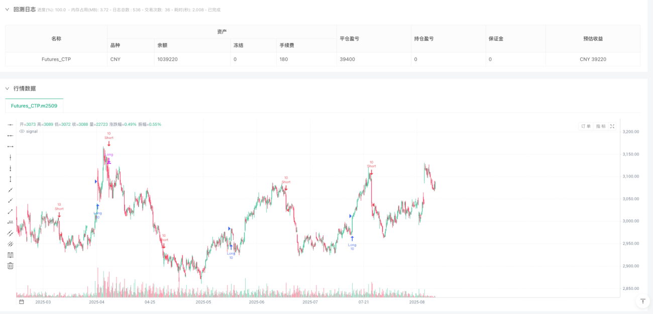
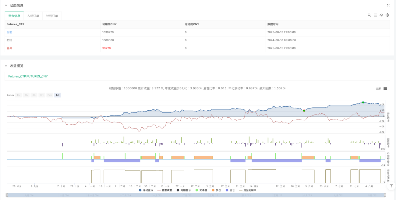
策略源码
/*backtest
start: 2024-08-18 09:00:00
end: 2025-08-17 15:00:00
period: 1h
basePeriod: 1h
exchanges: [{"eid":"Futures_CTP","currency":"FUTURES"}]
args: [["ContractType","m2509",360008]]
*/

// @version=6
strategy("Canuck Trading Traders Strategy [Candle Entropy Edition]", overlay=true, default_qty_value = 10)
// Note: Set Properties "Order size" to "100% of equity" for equity-based sizing or fixed contracts (e.g., 100).


// === CETP-Plus Settings ===
cetp_window = input.int(5, "CETP Window", minval=1, maxval=20, group="CETP-Plus Settings")
cetp_bins = input.int(3, "CETP Bins per Dimension", minval=1, maxval=10, group="CETP-Plus Settings")
long_threshold = input.float(0.1, "Long Threshold", minval=0.01, maxval=5.0, step=0.01, group="CETP-Plus Settings")
short_threshold = input.float(-0.1, "Short Threshold", minval=-0.8, maxval=-0.01, step=0.01, group="CETP-Plus Settings")
cetp_k = input.float(0.8, "CETP Momentum Weight", minval=0.1, maxval=5.0, step=0.1, group="CETP-Plus Settings")
mom_scale = input.float(6.0, "Momentum Scale", minval=1.0, maxval=20.0, step=1.0, group="CETP-Plus Settings")
body_weight = input.float(1.0, "Body Ratio Weight", minval=0.0, maxval=2.0, step=0.1, group="CETP-Plus Settings")
upper_weight = input.float(0.8, "Upper Wick Ratio Weight", minval=0.0, maxval=2.0, step=0.1, group="CETP-Plus Settings")
lower_weight = input.float(1.0, "Lower Wick Ratio Weight", minval=0.0, maxval=2.0, step=0.1, group="CETP-Plus Settings")
decay_factor = 0.8  // Hardcoded decay for exponential weighting (recent candles weighted more)

// === Trade Settings ===
min_score_strength = input.float(0.03, "Min CETP Score Strength", minval=0.0, maxval=5, step=0.01, group="Trade Settings")
stop_loss_pct = input.float(0.5, "Stop Loss (%)", minval=0.1, maxval=5.0, step=0.1, group="Trade Settings")
atr_mult = input.float(3.0, "ATR Multiplier", minval=0.5, maxval=10.0, step=0.1, group="Trade Settings")
trail_mult = input.float(5.0, "Trailing ATR Mult", minval=0.5, maxval=10.0, step=0.1, group="Trade Settings")
trail_offset_pct = input.float(1.0, "Trail Start Offset (%)", minval=0.5, maxval=10.0, step=0.1, group="Trade Settings")
min_price_move_mult = input.float(2.0, "Min Price Move ATR Mult (to avoid tiny trades)", minval=0.5, maxval=10.0, step=0.1, group="Trade Settings")  // Filter tiny moves

// Indicators (ATR for stops/trails only)
atr = nz(ta.atr(14), 0.0)

// Volatility Filter (CV < 15% to avoid chop)
vol_threshold = ta.stdev(close, 20) / ta.sma(close, 20) * 100
trade_allowed = vol_threshold < 15.0

// Minimum Price Move Filter (candle range > ATR multiple, floored by min tick)
min_price_move = math.max(atr * min_price_move_mult, syminfo.mintick * 10)  // Avoid sub-penny moves; 10x tick for robustness
price_move_condition = (high - low) > min_price_move  // Fixed: Use high - low instead of ta.range()

// CETP-Plus Calculation (Blended EMA, RSI, ATR, ADX theses)
epsilon = 1e-5
body_ratio = (close - open) / (high - low + epsilon) * body_weight
upper_wick_ratio = (high - math.max(open, close)) / (high - low + epsilon) * upper_weight
lower_wick_ratio = (math.min(open, close) - low) / (high - low + epsilon) * lower_weight

// EMA-like weighting: Exponentially weight recent candles with fixed-size rolling arrays
var float[] body_arr = array.new_float(cetp_window, 0.0)
var float[] upper_arr = array.new_float(cetp_window, 0.0)
var float[] lower_arr = array.new_float(cetp_window, 0.0)

// Shift and decay older values, add new at the end
for i = 0 to cetp_window - 2
    array.set(body_arr, i, array.get(body_arr, i + 1) * decay_factor)
    array.set(upper_arr, i, array.get(upper_arr, i + 1) * decay_factor)
    array.set(lower_arr, i, array.get(lower_arr, i + 1) * decay_factor)

array.set(body_arr, cetp_window - 1, body_ratio)
array.set(upper_arr, cetp_window - 1, upper_wick_ratio)
array.set(lower_arr, cetp_window - 1, lower_wick_ratio)

// Volatility scaling (ATR thesis)
bin_size = 2.0 / cetp_bins * (1 + atr / ta.sma(atr, 14))
hist_size = cetp_bins * cetp_bins * cetp_bins
var int[] hist = array.new_int(hist_size, 0)
array.fill(hist, 0)

for i = 0 to cetp_window - 1
    body_val = array.get(body_arr, i)
    upper_val = array.get(upper_arr, i)
    lower_val = array.get(lower_arr, i)
    
    body_bin = math.max(0, math.min(cetp_bins - 1, math.floor((body_val + 1) / bin_size)))
    upper_bin = math.max(0, math.min(cetp_bins - 1, math.floor((upper_val + 1) / bin_size)))
    lower_bin = math.max(0, math.min(cetp_bins - 1, math.floor((lower_val + 1) / bin_size)))
    
    bin_idx = body_bin * (cetp_bins * cetp_bins) + upper_bin * cetp_bins + lower_bin
    array.set(hist, bin_idx, array.get(hist, bin_idx) + 1)

entropy = 0.0
for i = 0 to hist_size - 1
    count = array.get(hist, i)
    p = count / cetp_window
    if p > 0
        entropy := entropy - p * math.log(p)

max_entropy = math.log(hist_size)
norm_entropy = max_entropy > 0 ? entropy / max_entropy : 0.0

// RSI-like momentum bias
avg_gain = ta.rma(math.max(close - close[1], 0), cetp_window)
avg_loss = ta.rma(math.max(close[1] - close, 0), cetp_window)
rsi_bias = avg_loss > 0 ? avg_gain / avg_loss : 1.0
momentum = ta.mom(close, cetp_window) / (close[cetp_window] != 0 ? close[cetp_window] : 1e-5)
momentum_adj = momentum * (1 + rsi_bias)

// ADX-like trend strength (automated and symmetric for bull/bear)
di_plus = ta.rma(math.max(high - high[1], 0), cetp_window) / atr
di_minus = ta.rma(math.max(low[1] - low, 0), cetp_window) / atr
trend_strength = di_plus > di_minus ? 1.2 : (di_minus > di_plus ? 1.2 : 1.0)

// CETP-Plus Score (optimized: no abs on momentum_adj to preserve sign for better short detection)
avg_body = nz(array.avg(body_arr), 0.0)
raw_score = avg_body * (1 - norm_entropy) * (cetp_k + momentum_adj * mom_scale)
cetp_score = nz(raw_score * trend_strength, 0.0)

// Position State
var float entry_price = na
var int bars_held = 0

if barstate.isconfirmed
    bars_held := strategy.position_size != 0 ? bars_held + 1 : 0

// Trade Logic: Rely solely on current CETP score for entries/exits/reversals, with min price move filter
if bar_index >= cetp_window and math.abs(cetp_score) > min_score_strength and trade_allowed and price_move_condition
    if cetp_score > long_threshold
        if strategy.position_size < 0
            strategy.close("Short", comment="Reverse to Long")
        if strategy.position_size <= 0
            strategy.entry("Long", strategy.long)
            entry_price := close
            sl = entry_price * (1 - stop_loss_pct / 100) - atr * atr_mult
            strategy.exit("Long Exit", "Long", stop=sl, trail_points=atr * trail_mult, trail_offset=entry_price * (trail_offset_pct / 100))
            bars_held := 1
    else if cetp_score < short_threshold
        if strategy.position_size > 0
            strategy.close("Long", comment="Reverse to Short")
        if strategy.position_size >= 0
            strategy.entry("Short", strategy.short)
            entry_price := close
            sl = entry_price * (1 + stop_loss_pct / 100) + atr * atr_mult
            strategy.exit("Short Exit", "Short", stop=sl, trail_points=atr * trail_mult, trail_offset=entry_price * (trail_offset_pct / 100))
            bars_held := 1