策略概述

多维博弈论交易策略是一种结合博弈论原理与技术分析的量化交易方法,主要通过识别市场参与者的群体行为、机构资金流向、流动性陷阱以及纳什均衡状态来寻找高概率交易机会。该策略基于这样一个核心理念:金融市场是不同参与者之间的博弈过程,通过分析这些参与者的行为模式和决策倾向,可以预测市场的潜在走向。策略采用自动化交易逻辑,结合动态风险管理系统,旨在捕捉由散户恐慌、机构资金流动以及流动性陷阱所造成的市场低效状态。

策略原理

该策略运用多层次的博弈论分析框架,通过以下四个关键维度对市场进行解析:

1. 群体行为检测:策略使用RSI指标(默认14周期)结合成交量分析来识别市场中的群体性恐慌或贪婪行为。当RSI超过70且成交量显著高于其20周期移动平均线(默认2倍)时,系统识别为散户群体性买入;当RSI低于30且同样伴随成交量异常时,则识别为散户群体性恐慌抛售。这些极端情况通常预示着市场可能出现逆转。

2. 流动性陷阱分析:策略扫描近期(默认50个周期)的高低点,寻找可能存在的"止损猎杀"区域。当价格突破近期高点但随后收盘于该高点下方,同时伴随成交量放大时,系统认为可能出现上行流动性陷阱;反之亦然。这些陷阱通常是由大型机构设置,目的是诱导散户触发止损单。

3. 机构资金流向分析:通过监测异常大的成交量(默认为均值的2.5倍)以及累积/分配指标(A/D线)来追踪机构活动。A/D线高于其21周期移动平均线且伴随大成交量被识别为机构累积行为;反之则为分配行为。此外,策略还使用Smart Money指数((收盘价-开盘价)/(最高价-最低价)*成交量)来确认聪明资金的方向。

4. 纳什均衡计算:策略基于价格的100周期移动平均线和标准差,计算出一个统计学意义上的"均衡带"。当价格位于这个均衡带内时,市场被视为处于稳定状态;当价格显著偏离均衡带时,则被视为过度买入或卖出状态,存在回归均衡的潜力。

基于上述四个维度的分析,策略生成三类交易信号:

• 逆势信号:当散户出现群体性抛售,同时伴随机构累积行为或下行流动性陷阱时,产生买入信号;反之产生卖出信号。
• 动量信号:当价格低于纳什均衡带,同时Smart Money指数为正且没有散户群体性买入时,产生买入信号;反之产生卖出信号。
• 均衡回归信号:当价格低于纳什均衡带且出现上涨趋势(收盘价高于前一周期)同时成交量高于均值时,产生买入信号;反之产生卖出信号。

最终的多维博弈论交易决策是综合这三类信号得出的,并通过基于minimax原则的动态仓位管理系统来调整风险暴露程度。

策略优势

1. 综合多维度市场信息:策略不仅关注价格和成交量等基础技术指标,还融入了市场参与者行为模式、机构资金流向、流动性陷阱和统计学均衡等多重因素,提供了对市场更全面的理解。

2. 适应不同市场条件:通过博弈论框架,策略能够在不同市场环境中自适应调整。在纳什均衡区域内,策略采取保守立场;在检测到机构活动时,策略更为激进;在散户恐慌时,策略采取逆势操作。

3. 动态风险管理:策略内置了完善的风险控制机制,包括自动止损(默认2%),目标获利(默认5%),以及基于市场状态的动态仓位调整,符合minimax原则,在保护资本的同时优化回报。

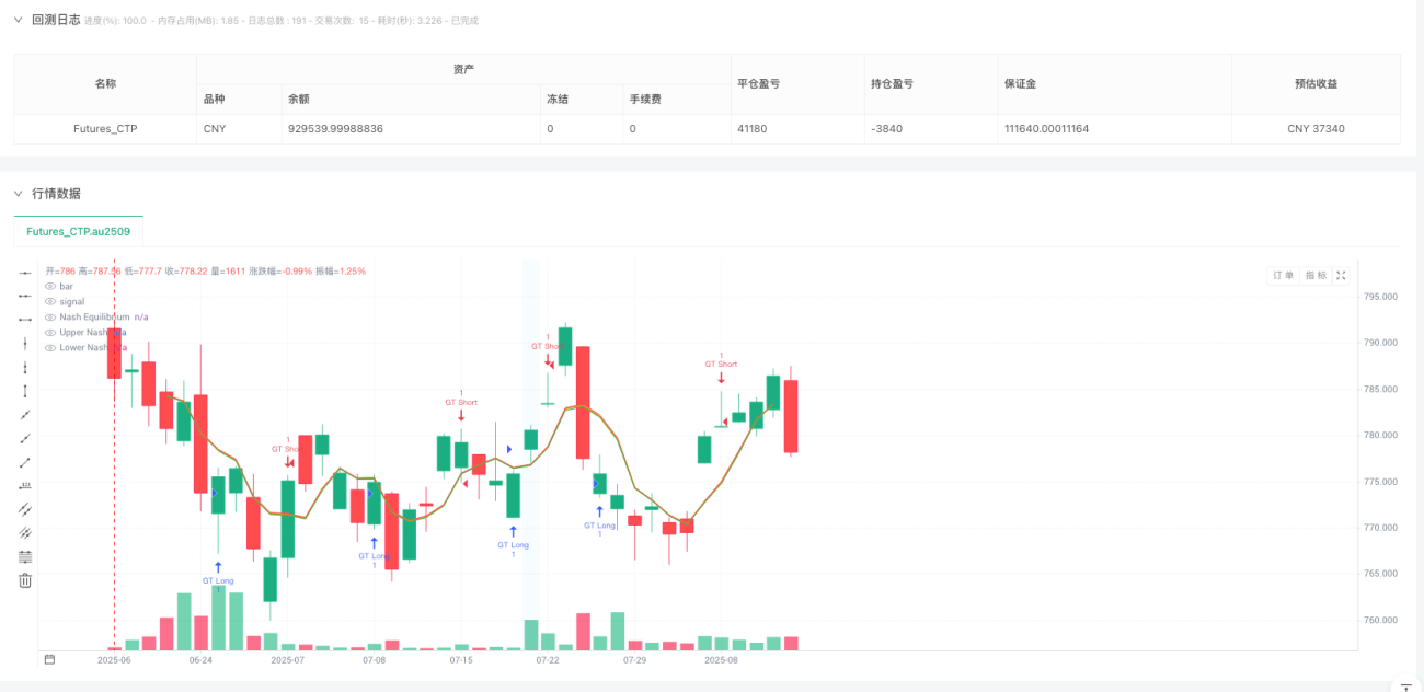
4. 可视化决策支持:策略提供了丰富的可视化元素,包括纳什均衡带、背景颜色指示器(红色表示群体买入,绿色表示群体卖出,蓝色表示机构活动),以及信号标记。同时,两个信息面板直观展示博弈论状态和回测性能数据。

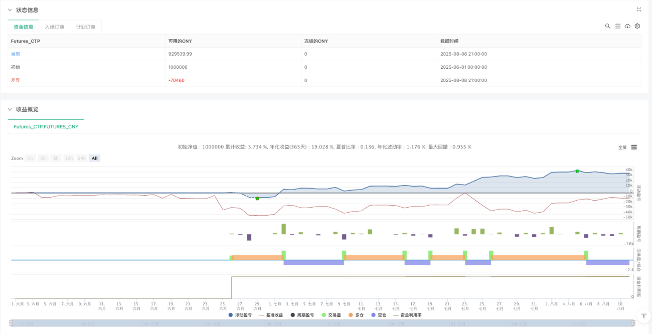
5. 完整的回测框架:策略内置全面的回测分析系统,追踪总交易次数、胜率、净利润、盈亏比、最大回撤等关键指标,便于策略优化和表现评估。

策略风险

1. 参数敏感性:策略的有效性高度依赖于各项参数的精确设置。RSI周期、成交量倍数阈值、流动性回溯期、纳什均衡偏差等参数需要根据不同市场和时间框架进行调整。不恰当的参数设置可能导致过多误信号或错过重要交易机会。

2. 市场噪音干扰:在短时间框架(如分钟级别)上,市场噪音可能导致群体行为和流动性陷阱的误判。策略最适合应用于H1(1小时)至D1(日线)等中长期时间框架,以过滤掉短期波动的干扰。

3. 过度交易风险:由于策略综合了三类信号源,在某些市场条件下可能产生过多交易信号,导致过度交易和手续费侵蚀。建议增加信号过滤机制,如信号确认期或强度阈值。

4. 系统性风险暴露:策略主要基于技术指标和行为分析,对宏观经济事件、政策变化或重大新闻等系统性风险因素缺乏适应性。在重大市场事件期间,策略可能无法正确评估风险并可能遭受重大损失。

5. 回测与实盘差异:回测结果可能存在前视偏差或过度拟合历史数据的问题。实盘交易中可能面临滑点、流动性不足或执行延迟等未在回测中体现的因素。

优化方向

1. 机器学习增强:引入机器学习算法来优化参数选择和信号生成过程。通过监督学习或强化学习方法,可以根据不同市场环境自动调整参数,提高策略的适应性和稳健性。

2. 多周期分析整合:在策略中增加多时间框架分析,例如同时考虑日线、4小时和1小时级别的信号,只有当多个时间框架信号一致时才执行交易,减少误信号和提高交易成功率。

3. 波动率调整机制:根据市场波动率动态调整止损水平、目标获利比例以及仓位大小。在高波动环境中收紧风险控制,在低波动环境中适度放宽参数,以适应不同市场条件。

4. 基本面数据整合:将宏观经济指标、市场情绪指数或新闻情绪分析纳入决策框架,创建一个更全面的交易系统,既考虑技术和行为因素,也考虑基本面因素。

5. 自适应过滤器:开发自适应信号过滤系统,根据历史信号表现动态调整信号阈值,过滤掉低概率交易机会,集中资源在高概率交易上,从而提高整体盈利能力和资本效率。

6. 纳什均衡改进:优化纳什均衡计算方法,考虑引入非线性统计模型或自适应均衡带宽度,使均衡判断更加准确,特别是在市场转换期或高波动期间。

总结

多维博弈论交易策略通过将经典博弈论原理与现代量化分析技术相结合,为交易者提供了一个独特的市场分析框架。该策略通过同时监测散户行为、机构活动、流动性陷阱和统计均衡状态,试图在混乱的市场中找到秩序,并从市场参与者之间的博弈中获取优势。

策略的核心优势在于其多维度分析能力和动态风险管理系统,使其能够适应不同市场环境并提供相对稳健的风险调整回报。然而,策略的复杂性也带来了参数优化的挑战和潜在的过度拟合风险。

对于希望应用此策略的交易者,建议首先在不同市场和时间框架上进行充分的回测,调整参数以适应特定交易品种的特性,并考虑引入本文提出的优化方向。此外,将本策略作为更广泛交易系统的一部分,而非单一决策依据,可能会取得更好的结果。

通过不断改进和优化,多维博弈论交易策略有潜力成为交易者工具箱中的有力武器,帮助在复杂多变的金融市场中获取持续的竞争优势。